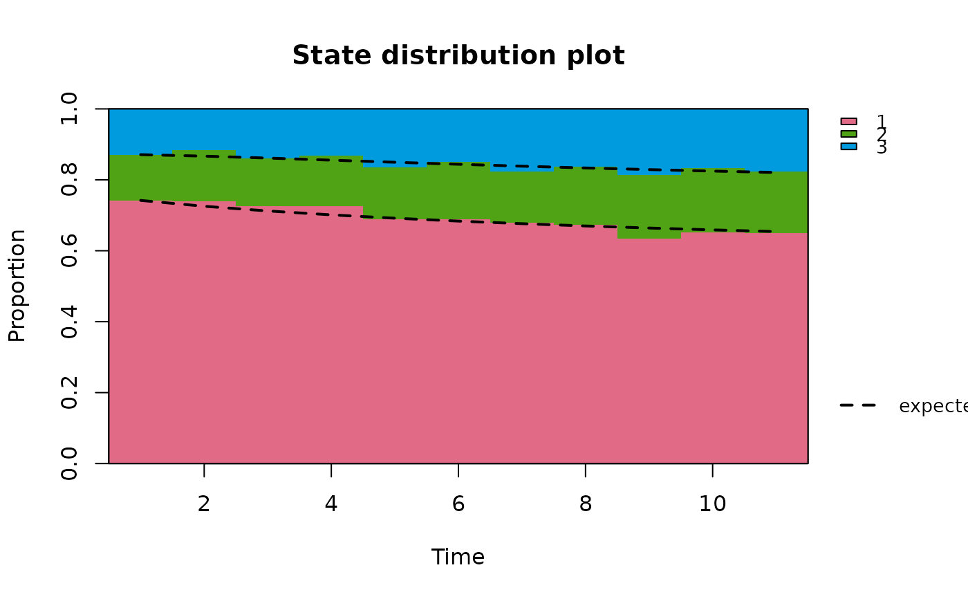
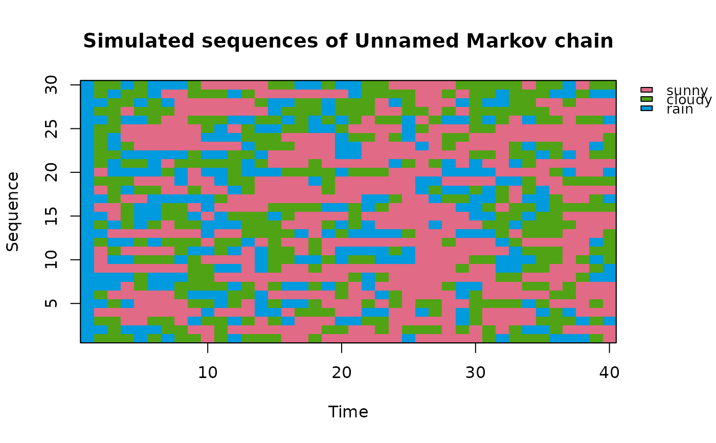
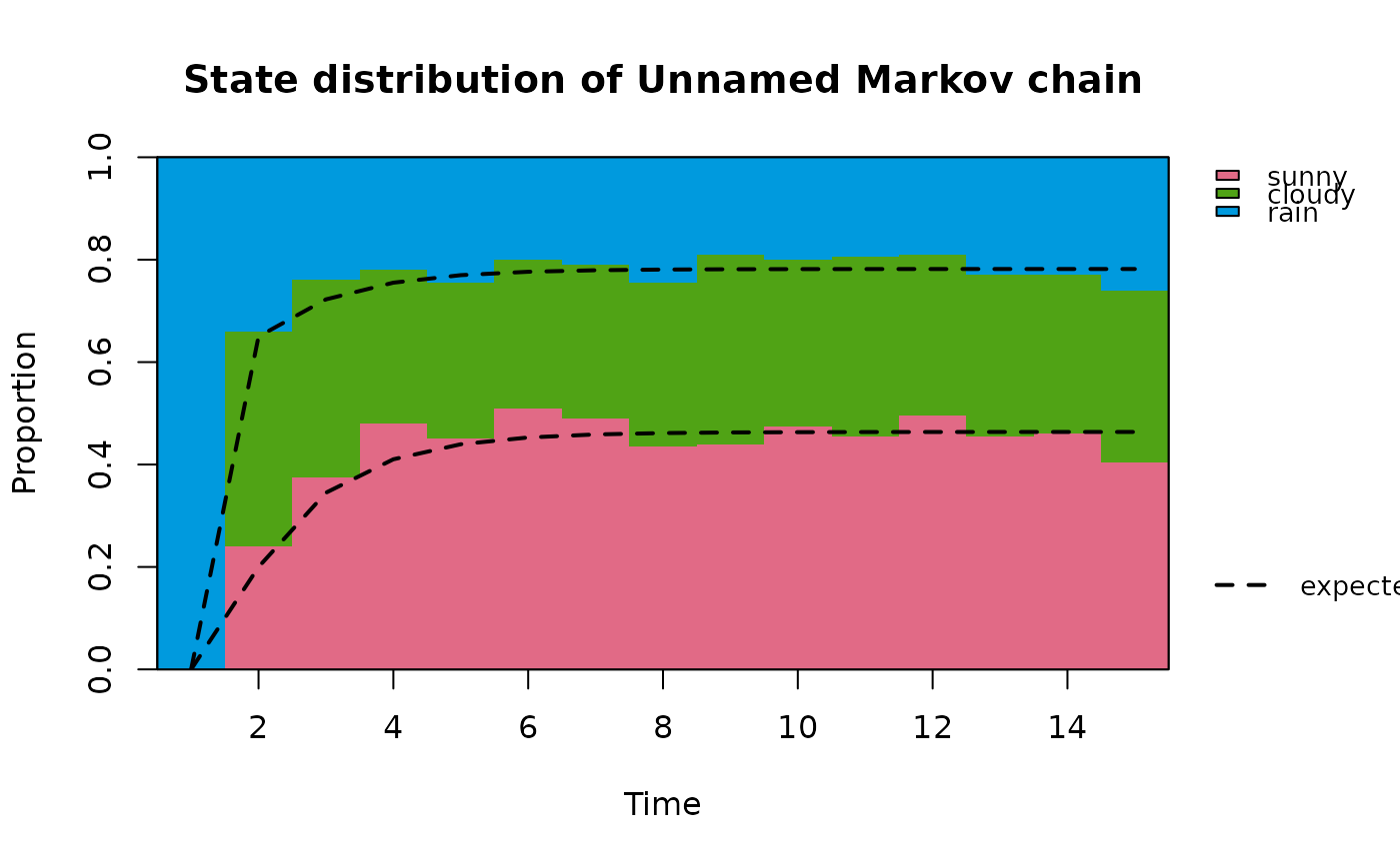
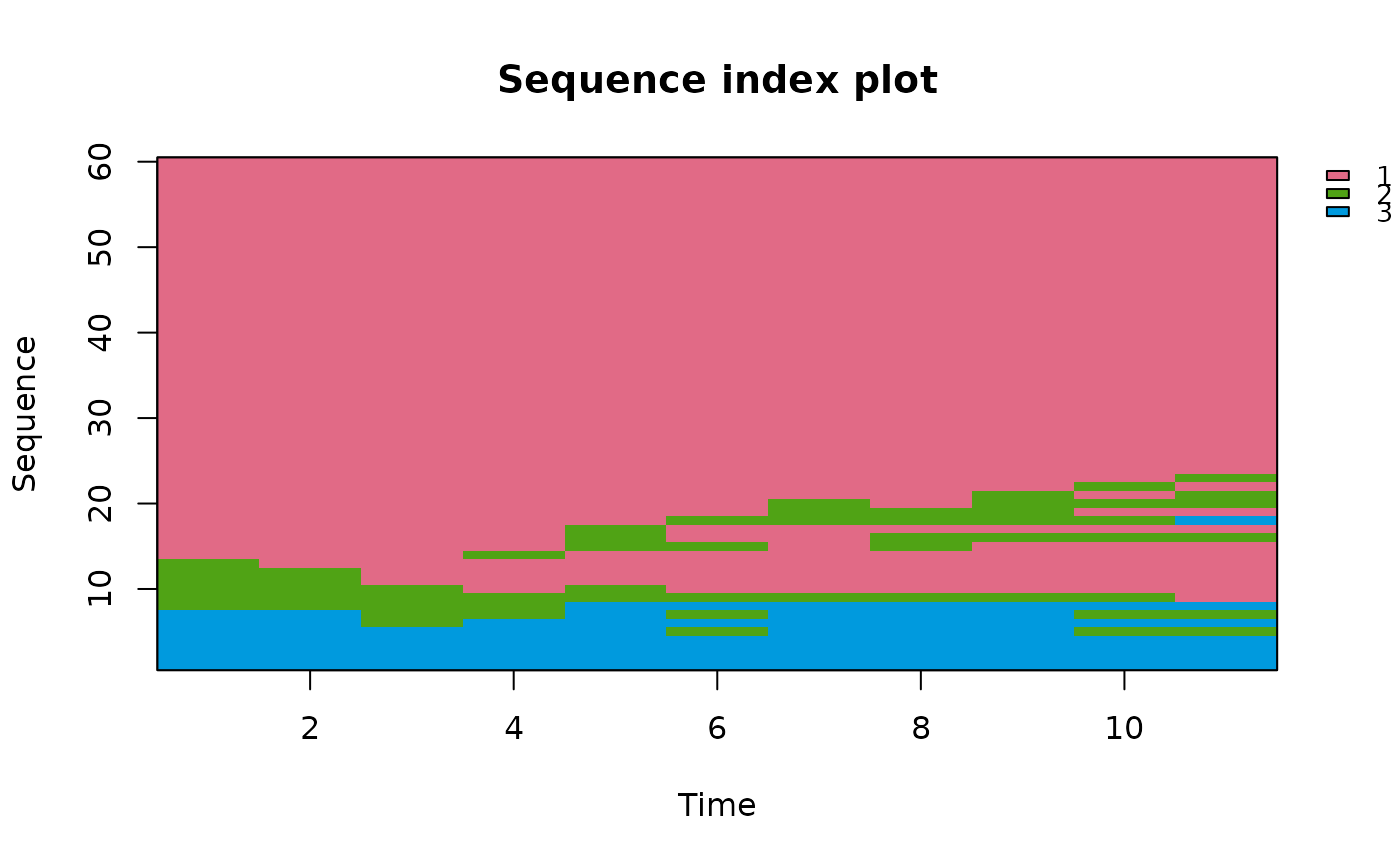
Plot state sequences of a Markov chain

Draws simulated or observed trajectories of a Markov chain either as a sequence index plot (each sequence a row of coloured cells, one per time point) or as a state distribution plot (the proportion of sequences in each state at each time point), optionally with the distribution expected from a chain overlaid.

Usage

plotSequence(
  x,
  type = c("index", "distribution"),
  nSequences = 20L,
  steps = 50L,
  initial = NULL,
  chain = NULL,
  sort = c("none", "first", "last"),
  expected = TRUE,
  col = NULL,
  legend = TRUE,
  main = NULL,
  xlab = "Time",
  ylab = NULL,
  seed = NULL,
  ...
)

Arguments

x: A markovchain object, from which nSequences sequences of steps time points are simulated, or observed data: a sequence, a list of sequences (of possibly different lengths), or a matrix or data frame with one sequence per row and one time point per column. Missing values are left blank.
type: "index" (the default) for a sequence index plot, "distribution" for a state distribution plot.
nSequences, steps: For a markovchain: the number of sequences to simulate and their number of time points (the initial state included).
initial: For a markovchain: the distribution of the initial state, as in redistribute: NULL (uniform, the default), a state name, or a numeric vector of probabilities.
chain: For observed data, an optional markovchain on the same states whose expected state distribution, started from the observed distribution at the first time point, is overlaid on the state distribution plot. For a markovchain x it is x itself.
sort: For type = "index": "none" (the default) keeps the sequences in their order; "first" and "last" sort them by their state at the first or last time point (ties broken by the following or preceding time points).
expected: For type = "distribution": whether to overlay the expected distribution when a chain is available (default TRUE).
col: Optional vector of colours, one per state. The default is grDevices::hcl.colors(n, "Dark 3").
legend: Whether to draw a legend of the states (default TRUE).
main, xlab, ylab: Title and axis labels.
seed: For a markovchain: an optional whole number. When given, the sequences are simulated after set.seed(seed) and the caller's random number stream is left untouched.
...: Further graphical parameters passed to plot.default.

Value

Invisibly, a list with sequences, the character matrix of the sequences as plotted (one row per sequence, after sorting); proportions, the matrix of the observed proportion of each state (rows) at each time point (columns); and expected, the matching matrix of expected proportions, or NULL when no chain is available.

Details

Sequence index plots and state distribution plots are the two basic graphs of sequence analysis (Gabadinho et al. 2011). For a Markov chain the first shows the lengths of the spells in each state and the second how the distribution of the state moves towards the stationary distribution. The expected distribution at time \(t\) is \(\mu_1 P^{t-1}\), with \(\mu_1\) the observed (or, for a markovchain x, the given) initial distribution, computed by redistribute; with observed data a systematic gap between the two suggests that the chain is not time-homogeneous (see assessStationarity). The proportions at each time point are computed over the sequences observed at that time point.

The sequences of a markovchain are simulated in C++ by inversion of the cumulative probabilities with R's uniform generator, so set.seed and seed control them. The plot is drawn with base graphics. The legend is placed in the right margin, which is widened for the purpose and restored afterwards.

References

Gabadinho, A., Ritschard, G., Mueller, N. S. and Studer, M. (2011). Analyzing and visualizing state sequences in R with TraMineR. Journal of Statistical Software, 40(4), 1-37. doi:10.18637/jss.v040.i04

Examples

s <- c("sunny", "cloudy", "rain")
weather <- new("markovchain", states = s, transitionMatrix = matrix(
  c(0.7, 0.2, 0.1, 0.3, 0.4, 0.3, 0.2, 0.45, 0.35), 3, byrow = TRUE,
  dimnames = list(s, s)))
plotSequence(weather, nSequences = 30, steps = 40, initial = "rain", seed = 1)

plotSequence(weather, type = "distribution", nSequences = 200, steps = 15,
             initial = "rain", seed = 1)


# observed trajectories, sorted by their first state, and their
# distribution against a time-homogeneous chain fitted to them
data(holson)
plotSequence(holson[1:60, 2:12], sort = "first")

fitted <- markovchainFit(holson[, 2:12])$estimate
plotSequence(holson[, 2:12], type = "distribution", chain = fitted)